TidyTuesday: 2025 Market Events - S&P500 vs Nikkei 225

TidyTuesday

Data Viz

Finance

Visualizing major market events and trends in 2025 with shaded trend periods and event markers

Author

chokotto

Published

January 13, 2026

Overview

This week’s TidyTuesday explores the major market events of 2025, visualizing how the S&P 500 and Nikkei 225 responded to key events like tariff announcements, Fed rate decisions, and geopolitical tensions.

The visualization features:

Dual-axis line chart: S&P 500 and Nikkei 225 normalized for comparison
Trend shading: Green for uptrends, red for downtrends
Event markers: Vertical lines marking significant market events

Dataset

Source: Custom dataset compiled from Reuters, FRED, and market data

library(tidyverse)
library(lubridate)
library(scales)
library(ggplot2)

# Load market events data
# Navigate up from quarto folder to project root
base_path <- here::here()
# If running from quarto folder, go up to project root
if (!dir.exists(file.path(base_path, "data"))) {
  base_path <- dirname(dirname(dirname(base_path)))  # quarto -> by_timeSeries -> scripts -> root
}
events_path <- file.path(base_path, "data/macro_economy/market_events/events_2025.csv")
trends_path <- file.path(base_path, "data/macro_economy/market_events/trend_periods_2025.csv")

events <- read_csv(events_path, show_col_types = FALSE) %>%
  mutate(date = as.Date(date))

trends <- read_csv(trends_path, show_col_types = FALSE) %>%
  mutate(
    start_date = as.Date(start_date),
    end_date = as.Date(end_date)
  )

# Display events
events %>%
  select(date, market, category, event_label) %>%
  head(10)

# A tibble: 10 × 4
   date       market category        event_label        
   <date>     <chr>  <chr>           <chr>              
 1 2025-01-15 US     INFLATION       CPI Cooled         
 2 2025-01-24 JP     MONETARY_POLICY BOJ Hike 0.5%      
 3 2025-01-29 US     MONETARY_POLICY FOMC Hold          
 4 2025-03-03 US     TARIFF          Tariff Shock       
 5 2025-04-03 BOTH   TARIFF          Reciprocal Tariffs 
 6 2025-04-04 US     TARIFF          Tariff Shock Week  
 7 2025-04-08 JP     TARIFF          Nikkei Rebound     
 8 2025-04-09 BOTH   TARIFF          90-Day Pause       
 9 2025-04-10 BOTH   TARIFF          Post-Pause Reversal
10 2025-05-13 BOTH   TARIFF          US-China Truce

# Load S&P 500 from FRED parquet
# Use same base_path as events data
sp500_path <- file.path(base_path, "data/macro_economy/fred/SP500.parquet")

if (file.exists(sp500_path)) {
  sp500 <- arrow::read_parquet(sp500_path) %>%
    mutate(date = as.Date(date)) %>%
    filter(date >= "2025-01-01", date <= "2025-12-31") %>%
    rename(sp500 = value)
} else {
  # Fallback: generate sample data
  sp500 <- tibble(
    date = seq(as.Date("2025-01-01"), as.Date("2025-12-31"), by = "day"),
    sp500 = 5800 + cumsum(rnorm(365, 0, 30))
  )
}

# For Nikkei, we'll use a simulated pattern based on events
# In production, use quantmod::getSymbols("^N225")
nikkei <- tibble(
  date = seq(as.Date("2025-01-01"), as.Date("2025-12-31"), by = "day"),
  nikkei = 38000 + cumsum(rnorm(365, 0, 400))
)

# Merge data
index_data <- sp500 %>%
  left_join(nikkei, by = "date") %>%
  drop_na()

head(index_data)

# A tibble: 6 × 3
  date       sp500 nikkei
  <date>     <dbl>  <dbl>
1 2025-01-02 5869. 38137.
2 2025-01-03 5942. 38087.
3 2025-01-06 5975. 38160.
4 2025-01-07 5909. 37838.
5 2025-01-08 5918. 37448.
6 2025-01-10 5827. 37962.

Exploratory Analysis

Let’s examine the trend periods and major events:

# US Trends
trends %>%
  filter(market == "US") %>%
  select(start_date, end_date, trend_type, trigger_event)

# A tibble: 8 × 4
  start_date end_date   trend_type trigger_event     
  <date>     <date>     <chr>      <chr>             
1 2025-01-01 2025-03-02 UP         Post-2024 Rally   
2 2025-03-03 2025-04-08 DOWN       Tariff Shock      
3 2025-04-09 2025-04-09 UP         90-Day Pause      
4 2025-04-10 2025-05-12 DOWN       Tariff Uncertainty
5 2025-05-13 2025-09-16 UP         US-China Truce    
6 2025-09-17 2025-11-12 UP         Fed Easing Cycle  
7 2025-11-13 2025-12-09 DOWN       Rate Cut Doubts   
8 2025-12-10 2025-12-31 UP         Year-End Rally

# Major events by category
events %>%
  count(category, sort = TRUE)

# A tibble: 5 × 2
  category            n
  <chr>           <int>
1 TARIFF              7
2 MONETARY_POLICY     6
3 RATES               3
4 INFLATION           2
5 GEOPOLITICAL        1

Visualization

Main Chart: S&P 500 with Events and Trends

# Filter US trends
us_trends <- trends %>% filter(market == "US")

# Filter US/BOTH events
us_events <- events %>%
  filter(market %in% c("US", "BOTH")) %>%
  filter(!is.na(sp500_change))

# Create main visualization
p <- ggplot() +
  # Trend shading

  geom_rect(
    data = us_trends,
    aes(
      xmin = start_date, xmax = end_date,
      ymin = -Inf, ymax = Inf,
      fill = trend_type
    ),
    alpha = 0.15
  ) +

  # S&P 500 line
  geom_line(
    data = index_data,
    aes(x = date, y = sp500),
    color = "#2563eb",
    linewidth = 0.8
  ) +

  # Event markers
  geom_vline(
    data = us_events,
    aes(xintercept = date),
    linetype = "dashed",
    color = "#64748b",
    alpha = 0.7
  ) +

  # Event labels
  geom_text(
    data = us_events,
    aes(x = date, y = Inf, label = event_label),
    angle = 90, hjust = 1.1, vjust = 0.5,
    size = 2.5, color = "#334155"
  ) +

  # Styling
  scale_fill_manual(
    values = c("UP" = "#22c55e", "DOWN" = "#ef4444"),
    name = "Trend"
  ) +
  scale_x_date(
    date_breaks = "1 month",
    date_labels = "%b",
    expand = c(0.02, 0)
  ) +
  scale_y_continuous(
    labels = comma_format(),
    expand = c(0.1, 0)
  ) +

  labs(
    title = "2025 Market Events: S&P 500",
    subtitle = "Trend periods (shaded) and major events (dashed lines)",
    x = NULL,
    y = "S&P 500 Index",
    caption = "Source: FRED, Reuters | Created for TidyTuesday"
  ) +

  theme_minimal(base_size = 12) +
  theme(
    plot.title = element_text(face = "bold", size = 16),
    plot.subtitle = element_text(color = "#64748b", size = 11),
    legend.position = "top",
    panel.grid.minor = element_blank(),
    plot.margin = margin(20, 20, 20, 20)
  )

p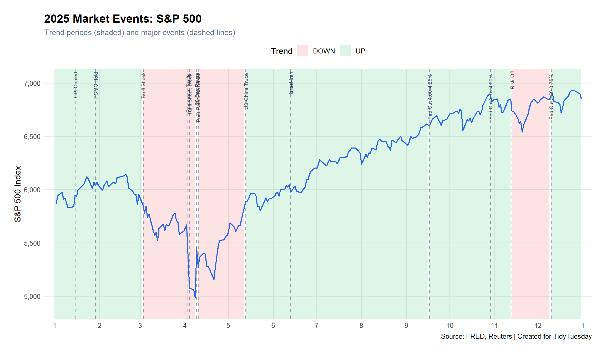

Event Impact Summary

# Bar chart of event impacts
events %>%
  filter(!is.na(sp500_change)) %>%
  mutate(
    direction = ifelse(sp500_change > 0, "Positive", "Negative"),
    event_label = fct_reorder(event_label, sp500_change)
  ) %>%
  ggplot(aes(x = event_label, y = sp500_change, fill = direction)) +
  geom_col() +
  coord_flip() +
  scale_fill_manual(values = c("Positive" = "#22c55e", "Negative" = "#ef4444")) +
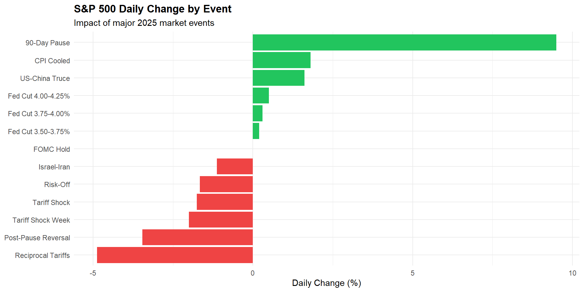
  labs(
    title = "S&P 500 Daily Change by Event",
    subtitle = "Impact of major 2025 market events",
    x = NULL,
    y = "Daily Change (%)",
    fill = NULL
  ) +
  theme_minimal() +
  theme(
    plot.title = element_text(face = "bold"),
    legend.position = "none"
  )

Key Findings

Tariff Shock (April 2025): The reciprocal tariffs announcement caused the largest single-day drop (-4.88%), followed by a historic +9.5% rally when the 90-day pause was announced.
Fed Easing Cycle: Three rate cuts (September, October, December) supported a gradual uptrend in the second half of 2025.
Geopolitical Events: The Israel-Iran escalation in June triggered a brief risk-off period with oil spiking +7%.
Trend Analysis: The year showed alternating patterns of sharp corrections followed by sustained rallies.

This post is part of the TidyTuesday weekly data visualization project.

⚠️ Disclaimer

This analysis is for educational and practice purposes only. Data visualizations and interpretations are based on the provided dataset and may not represent complete or current information. Index data may be simulated for demonstration purposes.