Show code
library(tidyverse)
library(scales)
library(glue)
library(patchwork)An Olympic schedule is not just a timetable — it’s a resource allocation problem made visible. This week’s TidyTuesday uses the complete event schedule for the 2026 Milan-Cortina Winter Olympics (1,866 events across 16 disciplines) to reveal the hidden structure: which days carry the heaviest load, where medal events cluster, and how training and competition rhythms overlap.
library(tidyverse)
library(scales)
library(glue)
library(patchwork)data_dir <- file.path(getwd(), "data")
schedule <- read_csv(file.path(data_dir, "schedule.csv"),
show_col_types = FALSE)
schedule <- schedule |>
mutate(
date = as.Date(date),
is_medal_event = as.logical(is_medal_event),
is_training = as.logical(is_training)
)
cat(glue(
"Total events: {nrow(schedule)}\n",
"Disciplines: {n_distinct(schedule$discipline_name)}\n",
"Venues: {n_distinct(schedule$venue_name)}\n",
"Date range: {min(schedule$date)} to {max(schedule$date)}\n",
"Medal events: {sum(schedule$is_medal_event)}\n",
"Training sessions: {sum(schedule$is_training)}"
))Total events: 1866
Disciplines: 16
Venues: 14
Date range: 2026-02-04 to 2026-02-22
Medal events: 344
Training sessions: 246NOTE_TEXT <- "Full event schedule including training and competition"
SOURCE_TEXT <- "TidyTuesday 2026-02-10 / Daniel Chen"
CAPTION <- glue("Note: {NOTE_TEXT} | Source: {SOURCE_TEXT} | \u00A9 2026 chokotto")
theme_fm <- theme_minimal(base_size = 12) +
theme(
plot.background = element_rect(fill = "white", color = NA),
panel.background = element_rect(fill = "#f8fafc", color = NA),
panel.grid.major = element_line(color = "#e2e8f0", linewidth = 0.3),
panel.grid.minor = element_blank(),
text = element_text(color = "#334155"),
axis.text = element_text(color = "#475569"),
plot.title = element_text(color = "#1e293b", face = "bold", size = 14),
plot.subtitle = element_text(color = "#64748b", size = 10),
plot.caption = element_text(
face = "italic", color = "#94a3b8", size = 9,
hjust = 0, margin = margin(t = 12)
),
plot.caption.position = "plot",
strip.text = element_text(color = "#1e293b", face = "bold"),
legend.background = element_rect(fill = "white", color = NA),
legend.text = element_text(color = "#475569"),
plot.margin = margin(15, 15, 15, 15)
)Where does the schedule concentrate? This heatmap shows total events per day per discipline — revealing the rhythm of the Games.
heatmap_data <- schedule |>
  count(date, discipline_name, name = "n_events") |>
  complete(date, discipline_name, fill = list(n_events = 0))

discipline_order <- schedule |>
  count(discipline_name) |>
  arrange(desc(n)) |>
  pull(discipline_name)

heatmap_data <- heatmap_data |>
  mutate(discipline_name = factor(discipline_name, levels = rev(discipline_order)))

p1 <- ggplot(heatmap_data, aes(x = date, y = discipline_name, fill = n_events)) +
  geom_tile(color = "white", linewidth = 0.4) +
  scale_fill_gradient(
    low = "#f1f5f9", high = "#e63946",
    name = "Events",
    breaks = c(0, 10, 20, 30, 40)
  ) +
  scale_x_date(
    date_labels = "%b %d",
    date_breaks = "2 days",
    expand = c(0, 0)
  ) +
  labs(
    title = "Olympic Event Density: Some Disciplines Run Every Day, Others Concentrate",
    subtitle = "Total events per day per discipline \u2014 darker = more events scheduled",
    caption = CAPTION,
    x = NULL,
    y = NULL
  ) +
  theme_fm +
  theme(
    axis.text.x = element_text(angle = 45, hjust = 1, size = 9),
    legend.position = "right",
    legend.key.height = unit(1.2, "cm")
  )

p1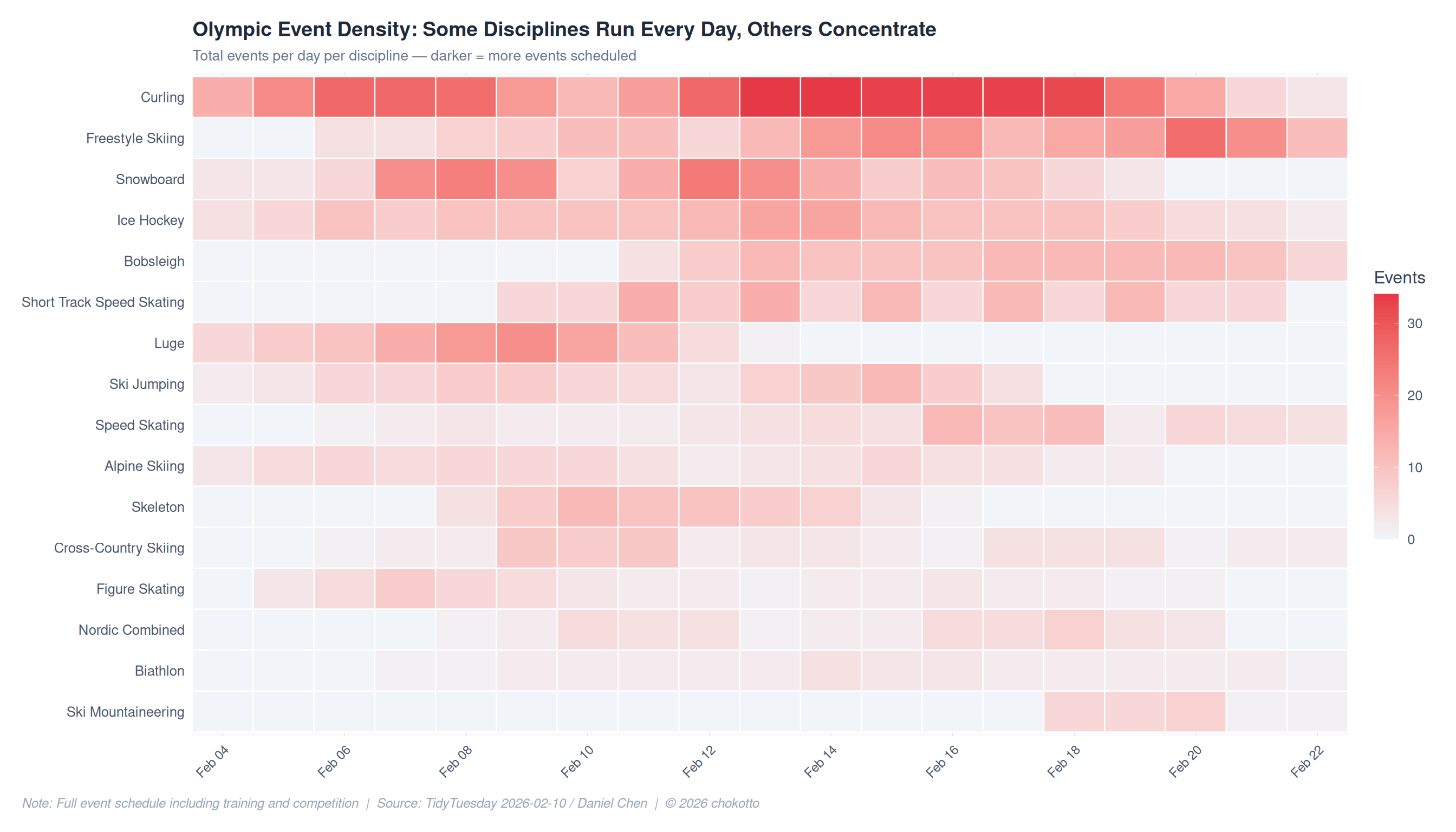
medal_by_date <- schedule |>
  filter(is_medal_event) |>
  count(date, name = "medal_events")

daily_total <- schedule |>
  filter(!is_training) |>
  count(date, name = "total_comp")

medal_context <- daily_total |>
  left_join(medal_by_date, by = "date") |>
  mutate(medal_events = replace_na(medal_events, 0),
         non_medal = total_comp - medal_events) |>
  pivot_longer(cols = c(medal_events, non_medal),
               names_to = "type", values_to = "count") |>
  mutate(type = factor(type, levels = c("non_medal", "medal_events"),
                       labels = c("Non-medal competition", "Medal events")))

p2 <- ggplot(medal_context, aes(x = date, y = count, fill = type)) +
  geom_col(width = 0.8) +
  scale_fill_manual(
    values = c("Non-medal competition" = "#94a3b8", "Medal events" = "#e63946"),
    name = NULL
  ) +
  scale_x_date(date_labels = "%b %d", date_breaks = "2 days") +
  scale_y_continuous(expand = expansion(mult = c(0, 0.05))) +
  labs(
    title = "Medal events peak mid-Games \u2014 the opening and closing days are lighter",
    subtitle = "Daily competition events split by medal / non-medal status",
    caption = CAPTION,
    x = NULL,
    y = "Events"
  ) +
  theme_fm +
  theme(
    legend.position = "top",
    legend.justification = "left"
  )

p2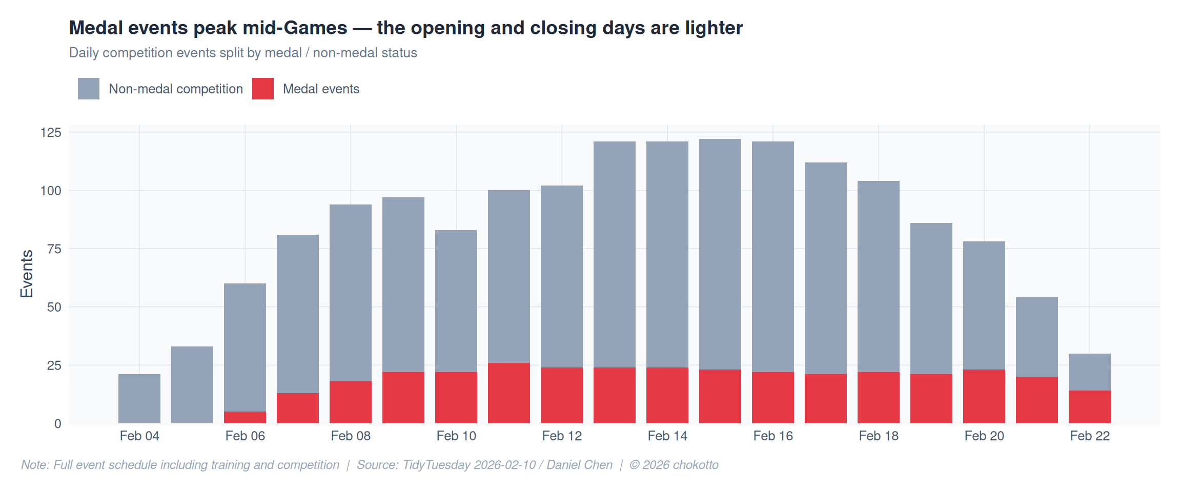
daily_type <- schedule |>
  mutate(session_type = if_else(is_training, "Training", "Competition")) |>
  count(date, session_type) |>
  mutate(session_type = factor(session_type, levels = c("Training", "Competition")))

p3 <- ggplot(daily_type, aes(x = date, y = n, fill = session_type)) +
  geom_area(alpha = 0.8, position = "stack") +
  scale_fill_manual(
    values = c("Training" = "#f59e0b", "Competition" = "#3b82f6"),
    name = NULL
  ) +
  scale_x_date(date_labels = "%b %d", date_breaks = "2 days") +
  scale_y_continuous(expand = expansion(mult = c(0, 0.05))) +
  labs(
    title = "Training sessions dominate early days, then competition takes over",
    subtitle = "Daily event volume by session type (stacked area)",
    caption = CAPTION,
    x = NULL,
    y = "Events"
  ) +
  theme_fm +
  theme(
    legend.position = "top",
    legend.justification = "left"
  )

p3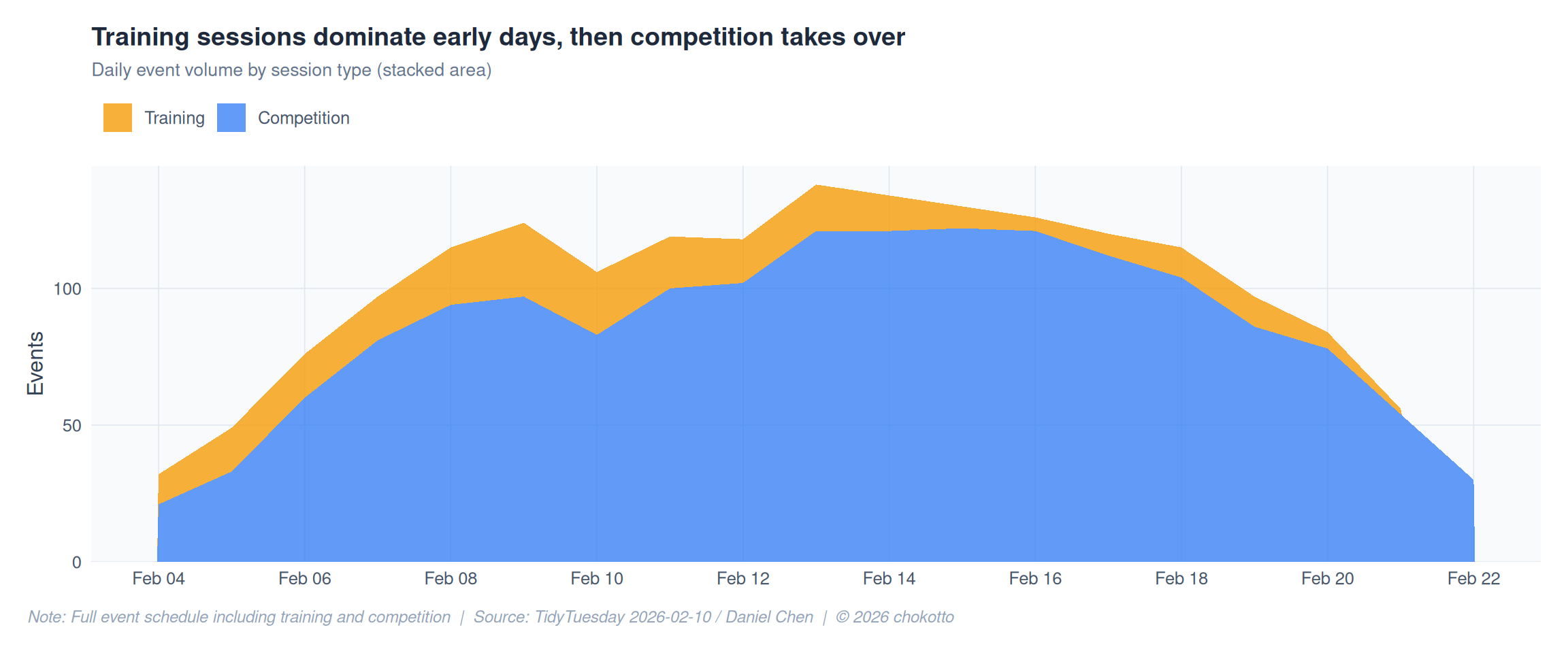
venue_summary <- schedule |>
  count(venue_name, sort = TRUE) |>
  mutate(venue_name = fct_reorder(venue_name, n))

venue_colors <- if_else(
  venue_summary$n == max(venue_summary$n), "#e63946", "#94a3b8"
)

p4 <- ggplot(venue_summary, aes(x = n, y = venue_name)) +
  geom_col(fill = venue_colors, width = 0.7) +
  geom_text(aes(label = n), hjust = -0.2, color = "#475569", size = 3.5) +
  scale_x_continuous(expand = expansion(mult = c(0, 0.15))) +
  labs(
    title = "Venue load is highly uneven \u2014 one venue hosts far more events than others",
    subtitle = "Total scheduled events by venue",
    caption = CAPTION,
    x = "Events",
    y = NULL
  ) +
  theme_fm

p4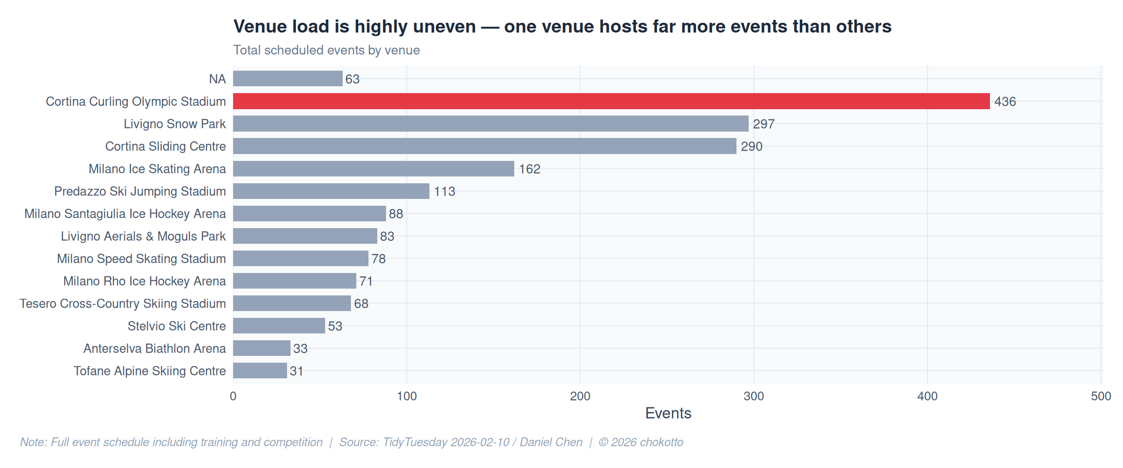
combined <- (p1 + labs(caption = NULL)) /
  (p2 + labs(caption = NULL)) /
  (p3 + labs(caption = NULL)) /
  (p4 + labs(caption = NULL)) +
  plot_layout(heights = c(2, 1, 1, 1)) +
  plot_annotation(
    title = "Milan-Cortina 2026: The Structure Behind the Schedule",
    subtitle = "1,866 events across 16 disciplines, 20 days, and multiple venues \u2014 when complexity peaks",
    caption = CAPTION,
    theme = theme(
      plot.background = element_rect(fill = "white", color = NA),
      plot.title = element_text(color = "#1e293b", face = "bold", size = 18),
      plot.subtitle = element_text(color = "#64748b", size = 12),
      plot.caption = element_text(
        face = "italic", color = "#94a3b8", size = 9,
        hjust = 0, margin = margin(t = 12)
      ),
      plot.caption.position = "plot"
    )
  )

combined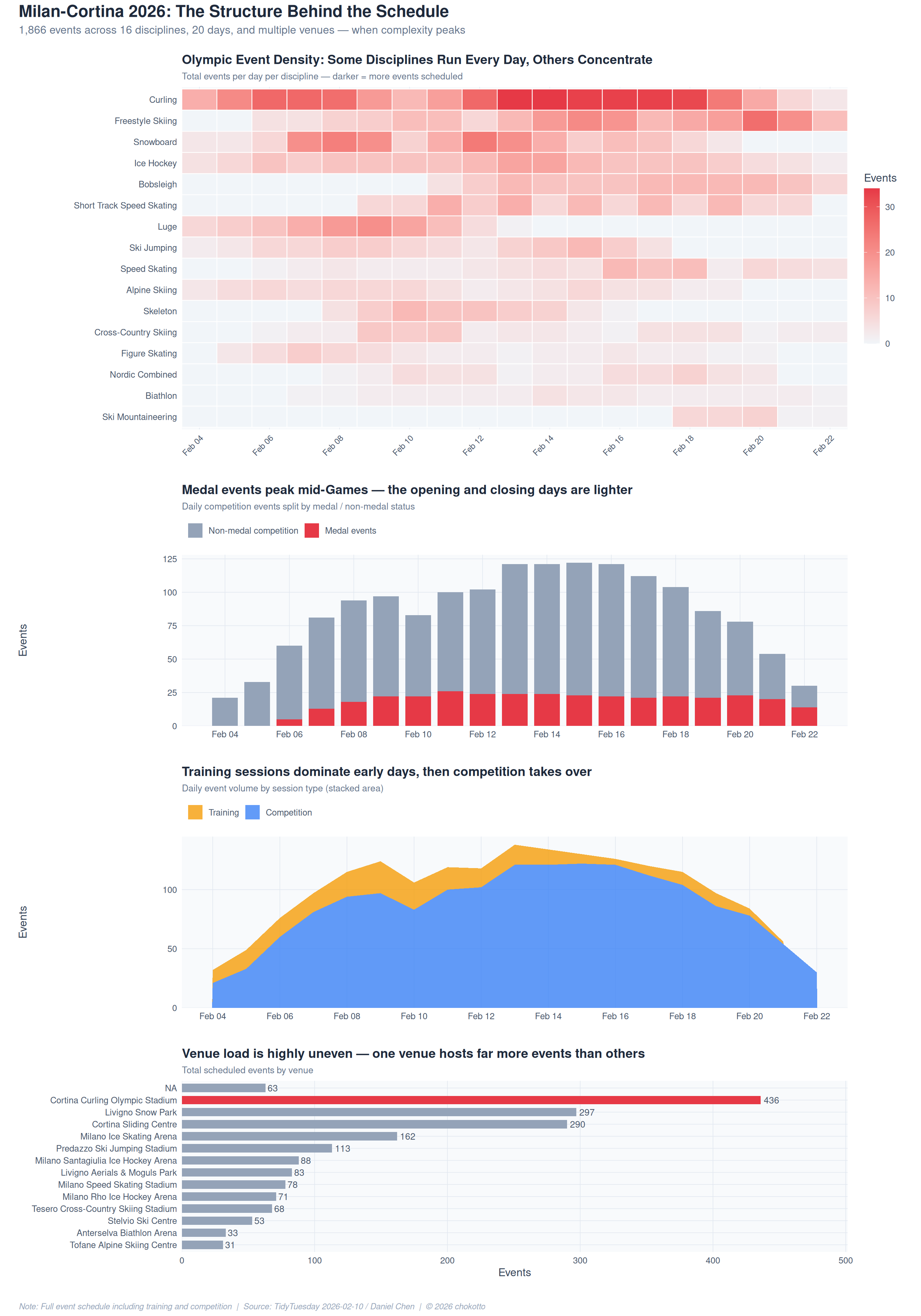
This post is part of the TidyTuesday weekly data visualization project.