Show code
library(tidyverse)
library(scales)
library(glue)
library(patchwork)Pi is infinite, irrational, and - supposedly - random in its digit distribution. But is it really? This week’s TidyTuesday provides the first one million digits of pi, letting us test that assumption visually. We look at four questions: are all digits equally common, how quickly does the distribution converge, what streak patterns emerge, and what does pi look like when you paint it on a grid?
digit_position (1-based index) + digit (0-9)library(tidyverse)
library(scales)
library(glue)
library(patchwork)data_dir <- file.path(getwd(), "data")
pi_digits <- read_csv(file.path(data_dir, "pi_digits.csv"),
show_col_types = FALSE)
cat(glue(
"Total digits: {nrow(pi_digits)}\n",
"Unique digits: {n_distinct(pi_digits$digit)}\n",
"First 20 digits: {paste(pi_digits$digit[1:20], collapse = '')}\n",
"Expected frequency per digit: {format(nrow(pi_digits) / 10, big.mark = ',')}"
))Total digits: 1000001
Unique digits: 10
First 20 digits: 31415926535897932384
Expected frequency per digit: 100,000.1NOTE_TEXT <- "First 1,000,001 digits of pi (including the leading 3)"
SOURCE_TEXT <- "TidyTuesday 2026-03-24 / Manasseh"
CAPTION <- glue("Note: {NOTE_TEXT} | Source: {SOURCE_TEXT} | \u00A9 2026 chokotto")
theme_fm <- theme_minimal(base_size = 12) +
theme(
plot.background = element_rect(fill = "white", color = NA),
panel.background = element_rect(fill = "#f8fafc", color = NA),
panel.grid.major = element_line(color = "#e2e8f0", linewidth = 0.3),
panel.grid.minor = element_blank(),
text = element_text(color = "#334155"),
axis.text = element_text(color = "#475569"),
plot.title = element_text(color = "#1e293b", face = "bold", size = 14),
plot.subtitle = element_text(color = "#64748b", size = 10),
plot.caption = element_text(
face = "italic", color = "#94a3b8", size = 9,
hjust = 0, margin = margin(t = 12)
),
plot.caption.position = "plot",
strip.text = element_text(color = "#1e293b", face = "bold"),
legend.background = element_rect(fill = "white", color = NA),
legend.text = element_text(color = "#475569"),
plot.margin = margin(15, 15, 15, 15)
)
ACCENT <- "#e63946"
BLUE <- "#3b82f6"
AMBER <- "#f59e0b"
GREEN <- "#10b981"
MUTED <- "#94a3b8"If pi’s digits are truly random, each digit (0-9) should appear exactly 10% of the time. With one million digits, the expected count per digit is 100,000. How close does reality get?
freq <- pi_digits |>
  count(digit) |>
  mutate(
    expected = nrow(pi_digits) / 10,
    deviation = n - expected,
    pct = n / nrow(pi_digits) * 100,
    fill_color = if_else(abs(deviation) == max(abs(deviation)), ACCENT,
                  if_else(deviation > 0, BLUE, MUTED))
  )

p1 <- ggplot(freq, aes(x = factor(digit), y = n, fill = fill_color)) +
  geom_col(width = 0.7) +
  geom_hline(yintercept = nrow(pi_digits) / 10,
             linetype = "dashed", color = ACCENT, linewidth = 0.6) +
  geom_text(aes(label = format(n, big.mark = ",")),
            vjust = -0.5, size = 3.5, color = "#475569") +
  scale_fill_identity() +
  scale_y_continuous(
    labels = label_comma(),
    expand = expansion(mult = c(0, 0.08))
  ) +
  annotate("text", x = 10.3, y = nrow(pi_digits) / 10,
           label = glue("Expected: {format(round(nrow(pi_digits)/10), big.mark = ',')}"),
           hjust = 0, size = 3, color = ACCENT, fontface = "italic") +
  labs(
    title = "Pi's digits are remarkably close to uniform - but not perfectly so",
    subtitle = glue("Digit frequency across {format(nrow(pi_digits), big.mark = ',')} digits | Max deviation: {format(max(abs(freq$deviation)), big.mark = ',')} from expected"),
    caption = CAPTION,
    x = "Digit", y = "Count"
  ) +
  coord_cartesian(clip = "off") +
  theme_fm +
  theme(legend.position = "none")

p1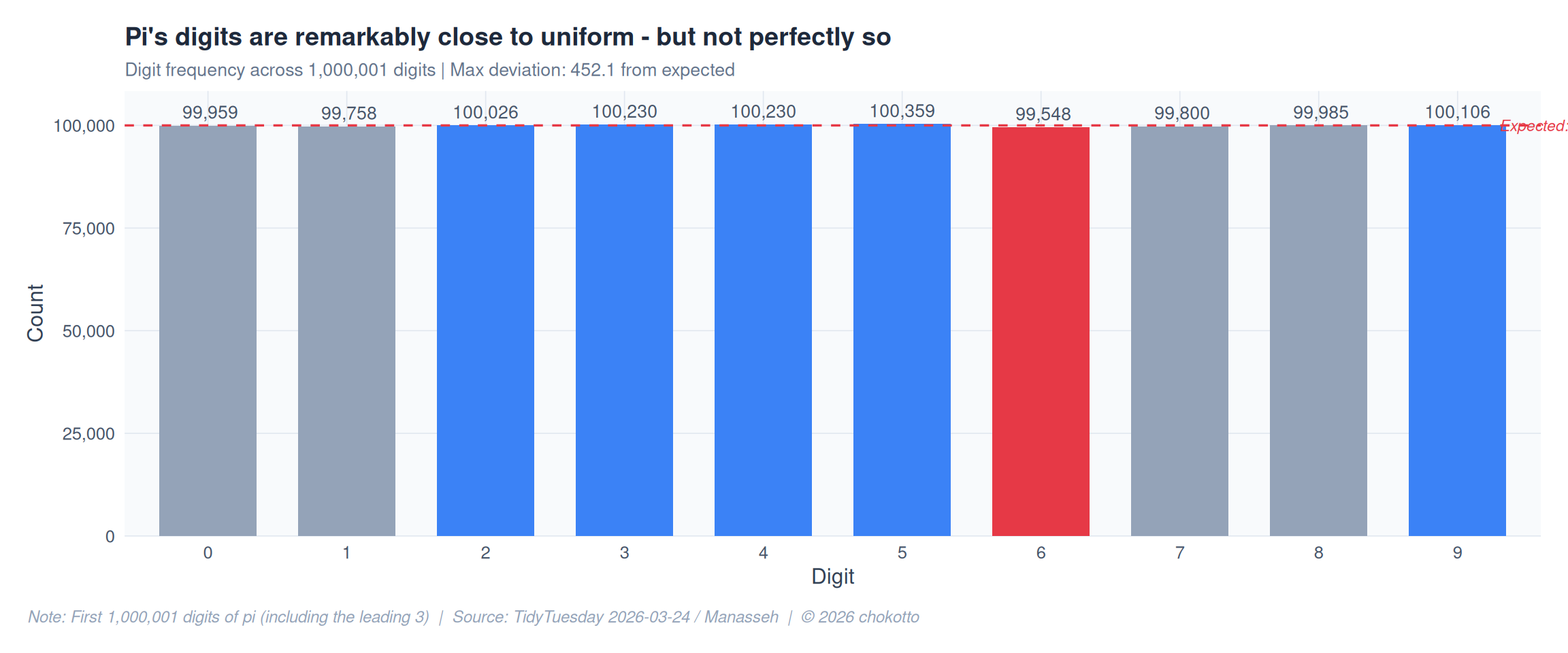
Starting from the first digit, track each digit’s running proportion. At what point do all ten lines settle near 10%?
sample_points <- c(
  seq(1, 100, by = 1),
  seq(100, 1000, by = 10),
  seq(1000, 10000, by = 100),
  seq(10000, 100000, by = 1000),
  seq(100000, 1000000, by = 10000)
) |> unique() |> sort()

convergence <- map_dfr(sample_points, function(n) {
  sub <- pi_digits |> slice(1:n)
  sub |>
    count(digit) |>
    complete(digit = 0:9, fill = list(n = 0)) |>
    mutate(
      sample_size = sum(n),
      proportion = n / sample_size
    ) |>
    select(digit, proportion, sample_size)
})

digit_colors <- c(
  "0" = MUTED, "1" = ACCENT, "2" = BLUE, "3" = GREEN, "4" = AMBER,
  "5" = "#8b5cf6", "6" = "#ec4899", "7" = "#14b8a6", "8" = "#f97316", "9" = "#6366f1"
)

p2 <- ggplot(convergence, aes(x = sample_size, y = proportion,
                               color = factor(digit), group = digit)) +
  geom_line(linewidth = 0.5, alpha = 0.8) +
  geom_hline(yintercept = 0.1, linetype = "dashed", color = "#cbd5e1", linewidth = 0.5) +
  scale_x_log10(
    labels = label_comma(),
    breaks = c(10, 100, 1000, 10000, 100000, 1000000)
  ) +
  scale_y_continuous(labels = label_percent(accuracy = 1),
                     limits = c(0, 0.5)) +
  scale_color_manual(values = digit_colors, name = "Digit") +
  labs(
    title = "By 10,000 digits all ten lines converge near 10% - but the first 100 are wild",
    subtitle = "Running proportion of each digit (0-9) as sample size grows (log scale)",
    caption = CAPTION,
    x = "Number of digits (log scale)", y = "Proportion"
  ) +
  theme_fm +
  theme(
    legend.position = "right",
    legend.key.size = unit(0.8, "lines")
  )

p2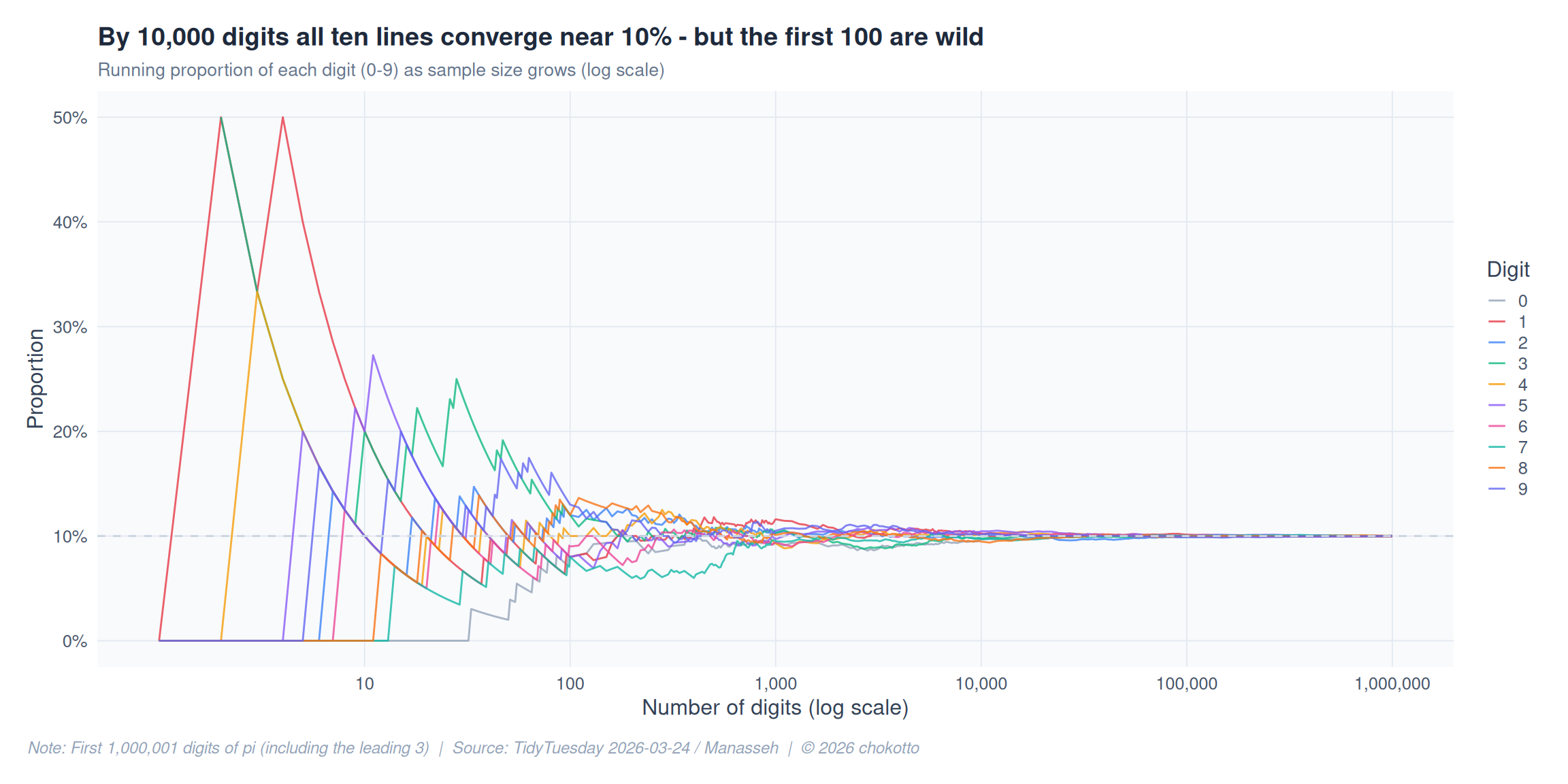
A streak is a consecutive run of the same digit (e.g., “111” = streak of 3). In truly random sequences, long streaks become exponentially rare.
runs <- rle(pi_digits$digit)
streaks <- tibble(
  digit = runs$values,
  length = runs$lengths
)

streak_dist <- streaks |>
  count(length, name = "occurrences") |>
  mutate(
    expected_theory = n_distinct(streaks$digit) * (0.1^(length - 1)) * 0.9 * nrow(streaks),
    fill_color = case_when(
      length >= 6 ~ ACCENT,
      length >= 4 ~ AMBER,
      TRUE ~ BLUE
    )
  )

longest <- streaks |> slice_max(length, n = 1, with_ties = FALSE)

p3 <- ggplot(streak_dist |> filter(length <= 10),
             aes(x = factor(length), y = occurrences, fill = fill_color)) +
  geom_col(width = 0.7) +
  geom_text(aes(label = format(occurrences, big.mark = ",")),
            vjust = -0.5, size = 3, color = "#475569") +
  scale_fill_identity() +
  scale_y_continuous(
    labels = label_comma(),
    expand = expansion(mult = c(0, 0.1))
  ) +
  labs(
    title = glue("Most streaks are just 1 digit long - the longest run is {longest$length} consecutive {longest$digit}s"),
    subtitle = "Distribution of consecutive same-digit run lengths in 1M digits of pi",
    caption = CAPTION,
    x = "Streak length (consecutive same digit)", y = "Occurrences"
  ) +
  theme_fm +
  theme(legend.position = "none")

p3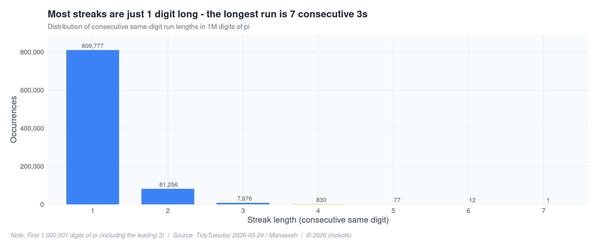
Each cell in this 100 x 100 grid represents one digit of pi (positions 2-10,001, after the leading 3), coloured by value. If pi were truly random, no visual pattern should emerge.
grid_n <- 10000
grid_data <- pi_digits |>
  slice(2:(grid_n + 1)) |>
  mutate(
    row = (row_number() - 1) %/% 100 + 1,
    col = (row_number() - 1) %% 100 + 1
  )

p4 <- ggplot(grid_data, aes(x = col, y = row, fill = factor(digit))) +
  geom_tile(width = 1, height = 1) +
  scale_fill_manual(
    values = c(
      "0" = "#f1f5f9", "1" = "#e63946", "2" = "#3b82f6", "3" = "#10b981",
      "4" = "#f59e0b", "5" = "#8b5cf6", "6" = "#ec4899", "7" = "#14b8a6",
      "8" = "#f97316", "9" = "#6366f1"
    ),
    name = "Digit"
  ) +
  scale_y_reverse() +
  coord_equal() +
  labs(
    title = "10,000 digits of pi as a colour grid - no visible pattern emerges",
    subtitle = "Each cell = one digit (row-major, positions 2-10,001) | 100 x 100 grid",
    caption = CAPTION
  ) +
  theme_fm +
  theme(
    axis.text = element_blank(),
    axis.title = element_blank(),
    panel.grid = element_blank(),
    legend.position = "right",
    legend.key.size = unit(0.6, "cm")
  )

p4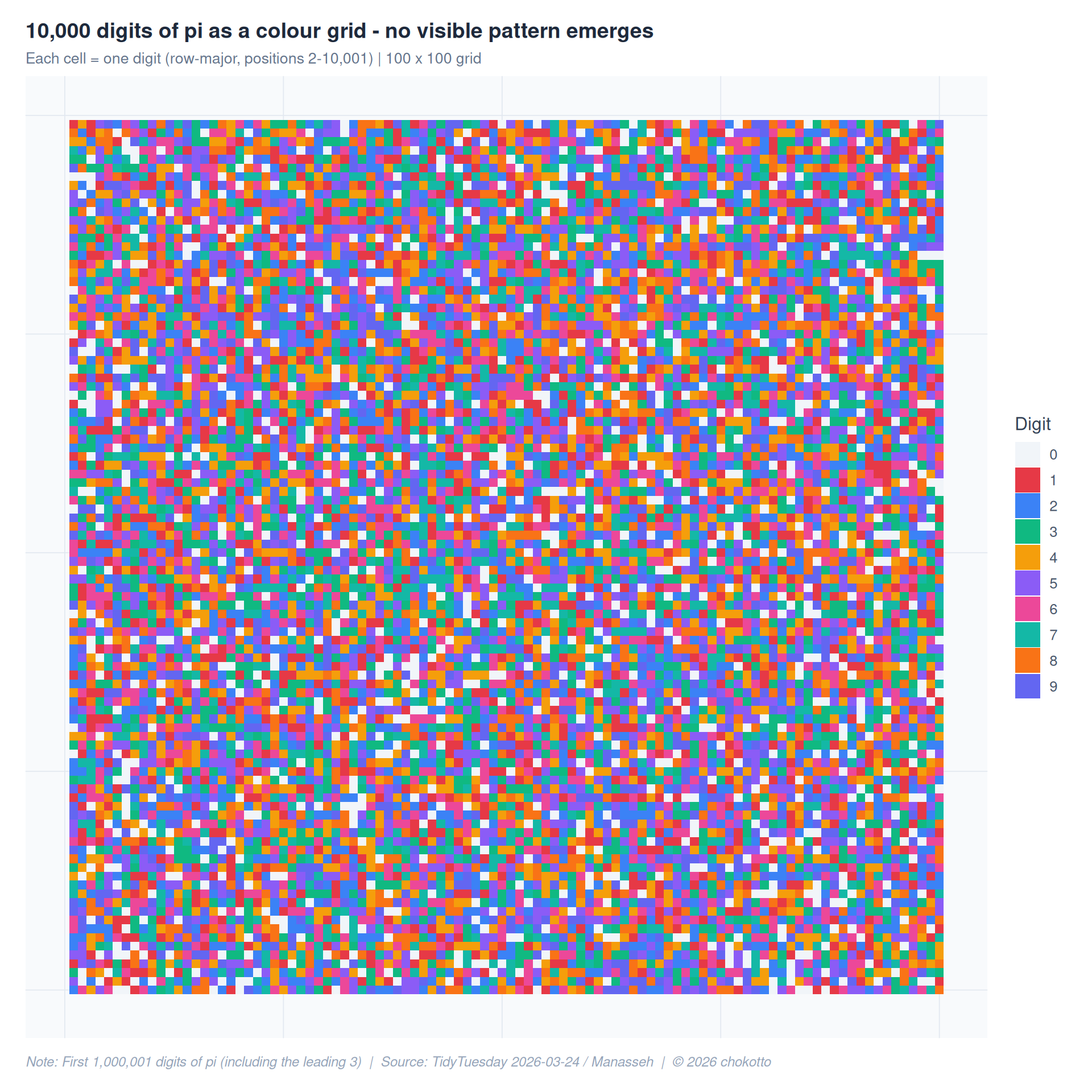
combined <- (p1 + labs(caption = NULL)) /
  (p2 + labs(caption = NULL)) /
  (p3 + labs(caption = NULL)) /
  (p4 + labs(caption = NULL)) +
  plot_layout(heights = c(1, 1.2, 1, 2)) +
  plot_annotation(
    title = "One Million Digits of Pi: Patterns in Randomness",
    subtitle = "Frequency, convergence, streaks, and visual structure in the first 1,000,001 digits",
    caption = CAPTION,
    theme = theme(
      plot.background = element_rect(fill = "white", color = NA),
      plot.title = element_text(color = "#1e293b", face = "bold", size = 18),
      plot.subtitle = element_text(color = "#64748b", size = 12),
      plot.caption = element_text(
        face = "italic", color = "#94a3b8", size = 9,
        hjust = 0, margin = margin(t = 12)
      ),
      plot.caption.position = "plot"
    )
  )

combined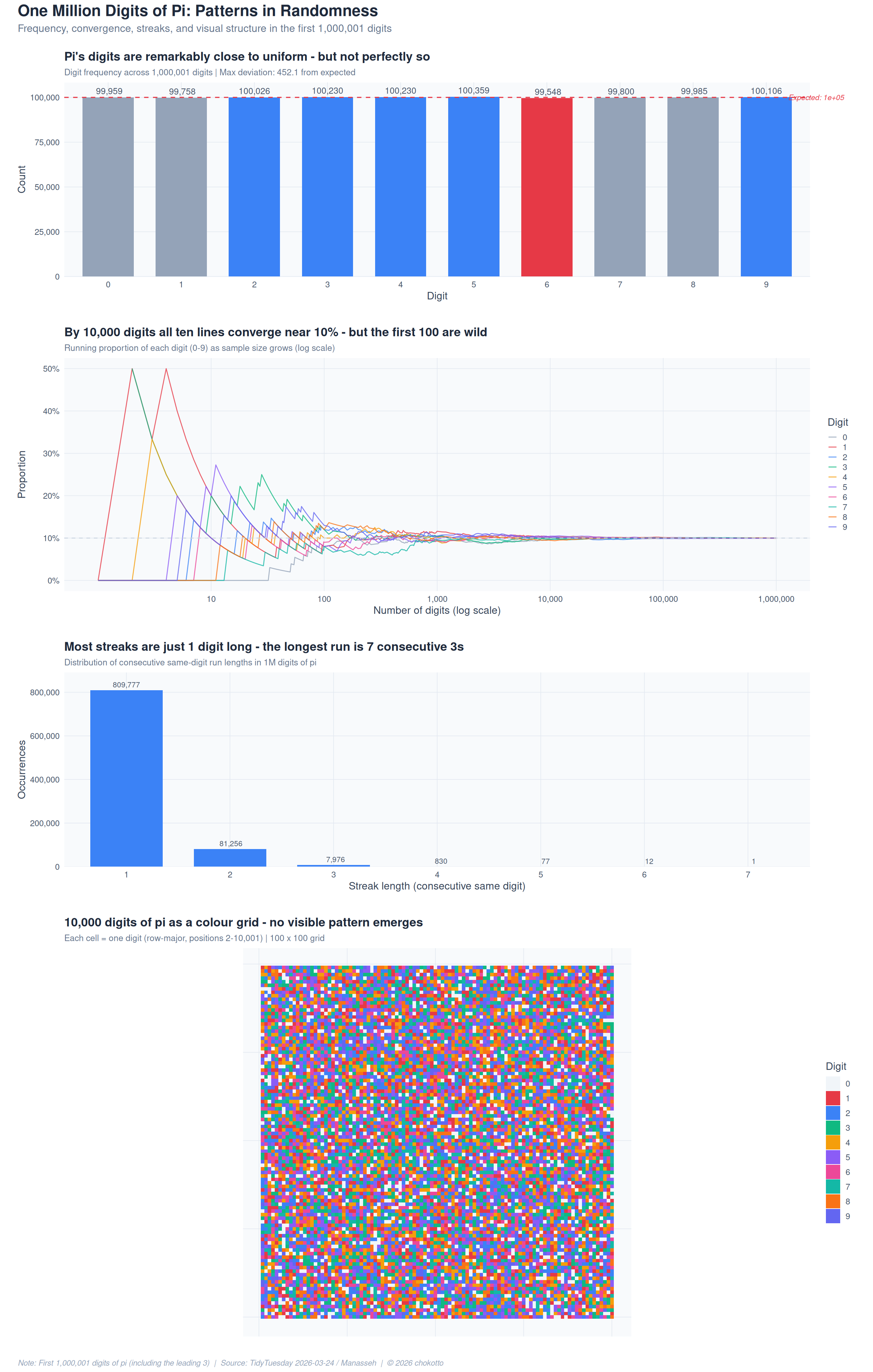
This post is part of the TidyTuesday weekly data visualization project.