Show code
library(tidyverse)
library(scales)
library(glue)
library(patchwork)The ocean does not warm uniformly. Surface waters respond quickly to atmospheric changes, while deeper layers lag behind – buffered by density, mixing, and stratification. This week’s TidyTuesday data lets us see that structure directly: 7 years of daily temperatures at 7 depths from a single coastal monitoring station in Nova Scotia, Canada.
The data comes from the Centre for Marine Applied Research (CMAR) Coastal Monitoring Program at Birchy Head, Lunenburg County. Sensors at depths from 2m to 40m recorded temperatures from February 2018 through December 2025.
library(tidyverse)
library(scales)
library(glue)
library(patchwork)data_dir <- file.path(getwd(), "data")
ocean_temp <- read_csv(file.path(data_dir, "ocean_temperature.csv"),
show_col_types = FALSE)
deployments <- read_csv(file.path(data_dir, "ocean_temperature_deployments.csv"),
show_col_types = FALSE)
ocean_temp <- ocean_temp |>
mutate(
date = as.Date(date),
year = year(date),
month = month(date),
month_name = month(date, label = TRUE),
depth_label = paste0(sensor_depth_at_low_tide_m, "m")
)
cat(glue(
"Records: {format(nrow(ocean_temp), big.mark = ',')}\n",
"Date range: {min(ocean_temp$date)} to {max(ocean_temp$date)}\n",
"Depths: {paste(sort(unique(ocean_temp$sensor_depth_at_low_tide_m)), collapse = ', ')}m\n",
"Years: {paste(sort(unique(ocean_temp$year)), collapse = ', ')}"
))Records: 19,165
Date range: 2018-02-20 to 2025-12-06
Depths: 2, 5, 10, 15, 20, 30, 40m
Years: 2018, 2019, 2020, 2021, 2022, 2023, 2024, 2025NOTE_TEXT <- "Daily mean temperature at Birchy Head, Nova Scotia (2018-2025)"
SOURCE_TEXT <- "TidyTuesday 2026-03-31 / CMAR Coastal Monitoring Program"
CAPTION <- glue("Note: {NOTE_TEXT} | Source: {SOURCE_TEXT} | \u00A9 2026 chokotto")
theme_fm <- theme_minimal(base_size = 12) +
theme(
plot.background = element_rect(fill = "white", color = NA),
panel.background = element_rect(fill = "#f8fafc", color = NA),
panel.grid.major = element_line(color = "#e2e8f0", linewidth = 0.3),
panel.grid.minor = element_blank(),
text = element_text(color = "#334155"),
axis.text = element_text(color = "#475569"),
plot.title = element_text(color = "#1e293b", face = "bold", size = 14),
plot.subtitle = element_text(color = "#64748b", size = 10),
plot.caption = element_text(
face = "italic", color = "#94a3b8", size = 9,
hjust = 0, margin = margin(t = 12)
),
plot.caption.position = "plot",
strip.text = element_text(color = "#1e293b", face = "bold"),
legend.background = element_rect(fill = "white", color = NA),
legend.text = element_text(color = "#475569"),
plot.margin = margin(15, 15, 15, 15)
)
ACCENT <- "#e63946"
BLUE <- "#3b82f6"
AMBER <- "#f59e0b"
GREEN <- "#10b981"
MUTED <- "#94a3b8"The heatmap below shows every day and every depth. The seasonal pulse is unmistakable at the surface, but it fades and compresses with depth – the ocean’s thermal inertia made visible.
p1 <- ocean_temp |>
  ggplot(aes(x = date, y = factor(sensor_depth_at_low_tide_m),
             fill = mean_temperature_degree_c)) +
  geom_tile(width = 1) +
  scale_fill_viridis_c(
    option = "turbo",
    name = "Temp (\u00B0C)",
    limits = c(-1, 22),
    breaks = seq(0, 20, by = 5)
  ) +
  scale_x_date(
    date_breaks = "1 year",
    date_labels = "%Y",
    expand = c(0.01, 0)
  ) +
  scale_y_discrete(limits = rev(c("2", "5", "10", "15", "20", "30", "40")),
                   labels = function(x) paste0(x, "m")) +
  labs(
    title = "Surface waters swing 20\u00B0C across seasons -- deep layers barely move",
    subtitle = "Daily mean temperature by depth at Birchy Head, Nova Scotia (2018-2025)",
    caption = CAPTION,
    x = NULL, y = "Depth"
  ) +
  theme_fm +
  theme(
    legend.position = "right",
    panel.grid.major = element_blank()
  )

p1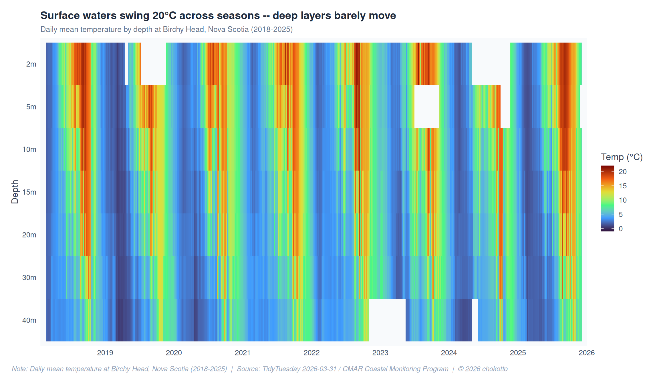
By averaging across years, we can isolate the seasonal cycle at each depth. Surface waters (2m) reach 18-20 degrees C in summer, while the 40m layer stays below 8 degrees C year-round.
seasonal <- ocean_temp |>
  group_by(month, sensor_depth_at_low_tide_m) |>
  summarise(
    mean_temp = mean(mean_temperature_degree_c, na.rm = TRUE),
    sd_temp = sd(mean_temperature_degree_c, na.rm = TRUE),
    .groups = "drop"
  )

depth_colors <- setNames(
  viridisLite::viridis(7, option = "viridis"),
  c("2", "5", "10", "15", "20", "30", "40")
)

p2 <- seasonal |>
  ggplot(aes(x = month, y = mean_temp,
             color = factor(sensor_depth_at_low_tide_m),
             group = factor(sensor_depth_at_low_tide_m))) +
  geom_ribbon(aes(ymin = mean_temp - sd_temp, ymax = mean_temp + sd_temp,
                  fill = factor(sensor_depth_at_low_tide_m)),
              alpha = 0.1, color = NA) +
  geom_line(linewidth = 1.2) +
  geom_point(size = 1.5) +
  scale_x_continuous(breaks = 1:12, labels = month.abb) +
  scale_color_manual(values = depth_colors, name = "Depth",
                     labels = function(x) paste0(x, "m")) +
  scale_fill_manual(values = depth_colors, guide = "none") +
  labs(
    title = "Summer warmth barely penetrates below 20m -- the deep stays cold year-round",
    subtitle = "Monthly mean temperature by depth (ribbon = +/- 1 SD across years)",
    caption = CAPTION,
    x = NULL, y = "Temperature (\u00B0C)"
  ) +
  theme_fm +
  theme(legend.position = "right")

p2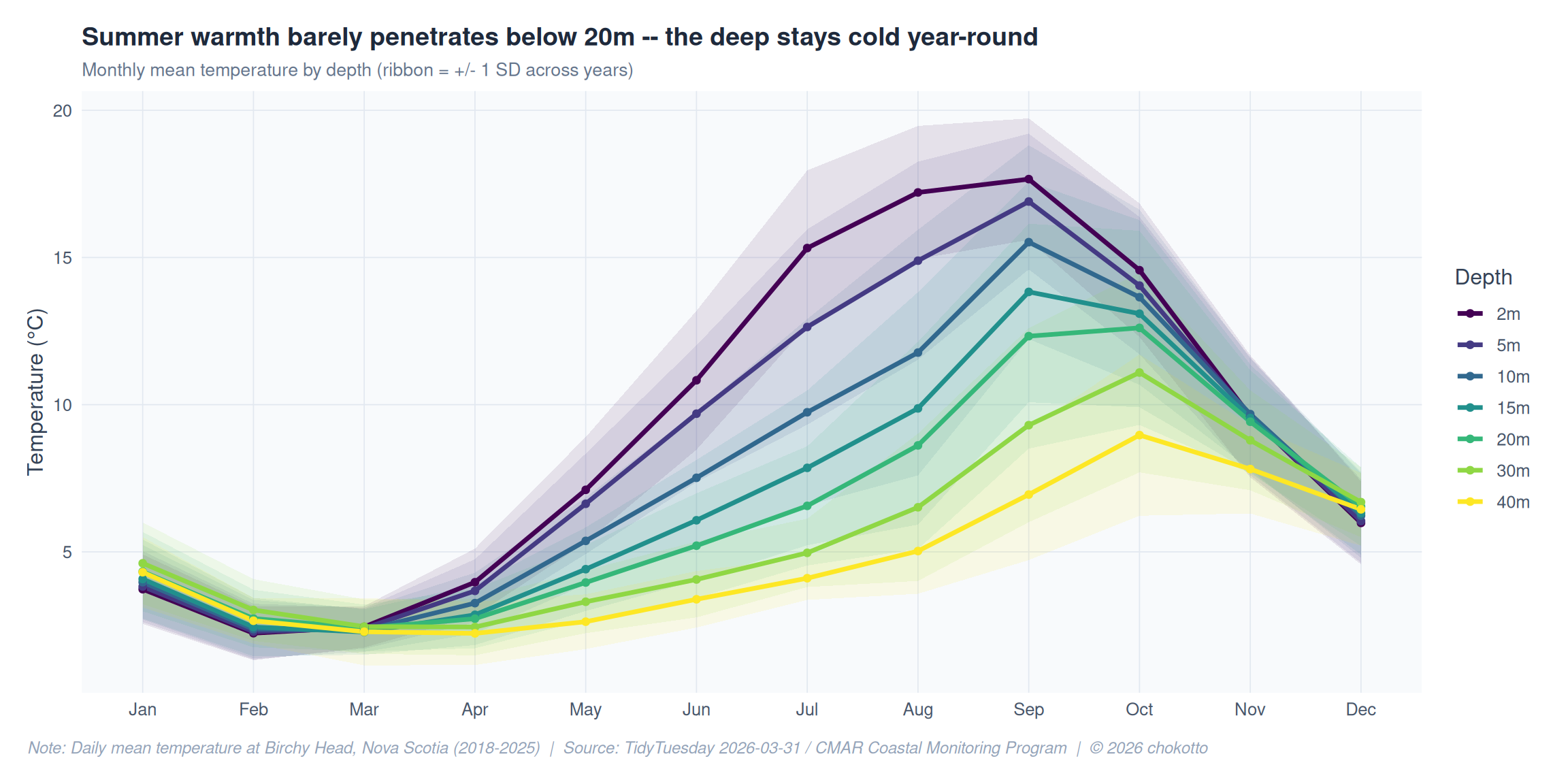
Comparing annual means by depth reveals whether warming is uniform or concentrated at the surface.
annual <- ocean_temp |>
  filter(month >= 3 & month <= 11) |>
  group_by(year, sensor_depth_at_low_tide_m) |>
  summarise(mean_temp = mean(mean_temperature_degree_c, na.rm = TRUE),
            .groups = "drop")

highlight_depths <- c(2, 20, 40)
annual_highlight <- annual |>
  filter(sensor_depth_at_low_tide_m %in% highlight_depths)

p3 <- annual |>
  ggplot(aes(x = year, y = mean_temp,
             group = factor(sensor_depth_at_low_tide_m))) +
  geom_line(color = MUTED, alpha = 0.3, linewidth = 0.8) +
  geom_line(data = annual_highlight,
            aes(color = factor(sensor_depth_at_low_tide_m)),
            linewidth = 1.4) +
  geom_point(data = annual_highlight,
             aes(color = factor(sensor_depth_at_low_tide_m)),
             size = 2.5) +
  scale_color_manual(
    values = c("2" = ACCENT, "20" = BLUE, "40" = "#440154"),
    name = "Depth",
    labels = function(x) paste0(x, "m")
  ) +
  scale_x_continuous(breaks = 2018:2025) +
  labs(
    title = "Surface and mid-depth temperatures show more year-to-year variability than the deep",
    subtitle = "Annual mean temperature (Mar-Nov) by depth | Grey = other depths",
    caption = CAPTION,
    x = NULL, y = "Temperature (\u00B0C)"
  ) +
  theme_fm +
  theme(legend.position = "right")

p3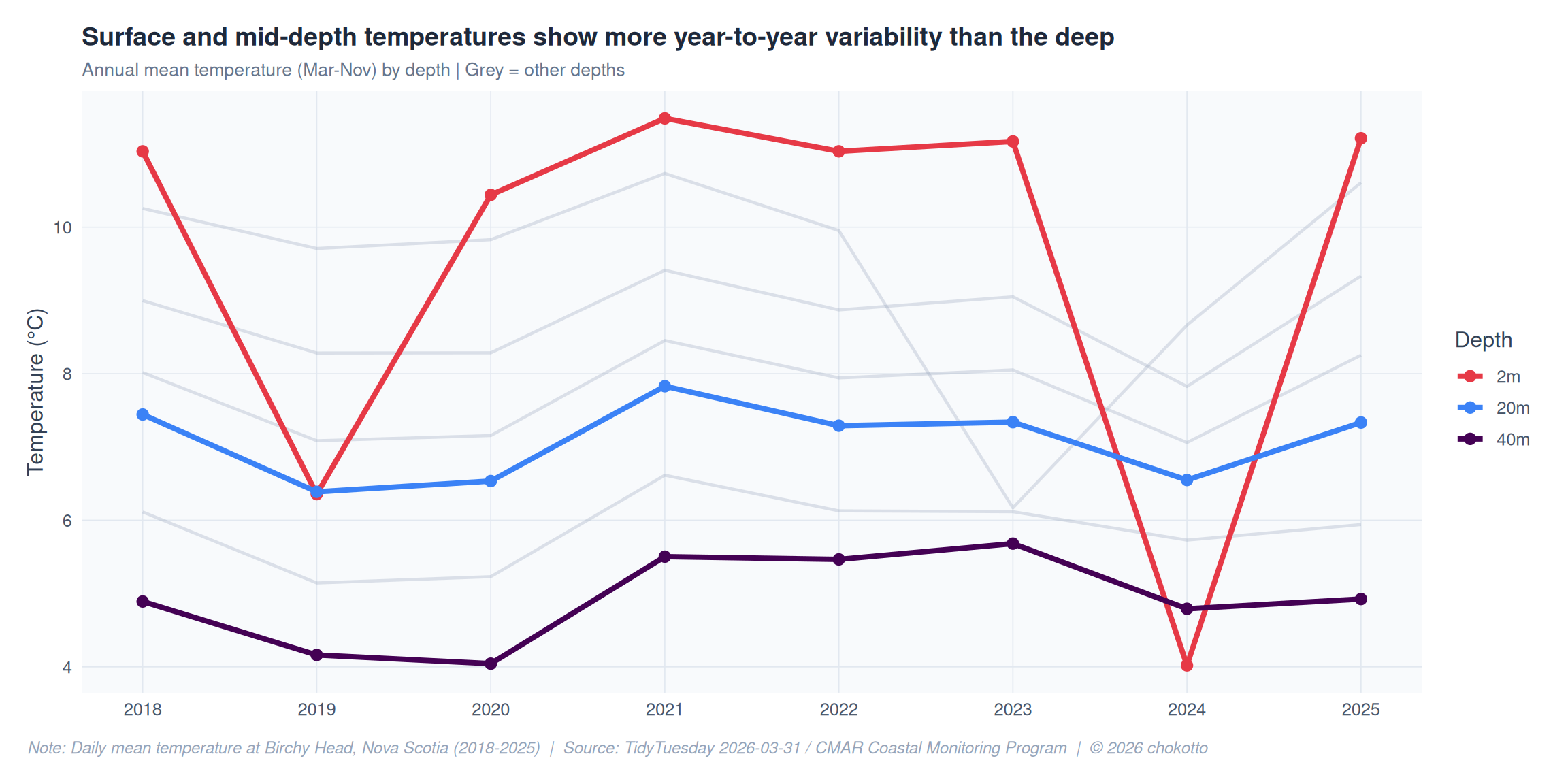
Standard deviation of daily temperatures reveals where the ocean is most variable – and where it is remarkably stable.
variability <- ocean_temp |>
  group_by(sensor_depth_at_low_tide_m) |>
  summarise(
    mean_sd = mean(sd_temperature_degree_c, na.rm = TRUE),
    overall_sd = sd(mean_temperature_degree_c, na.rm = TRUE),
    .groups = "drop"
  ) |>
  mutate(
    depth_label = paste0(sensor_depth_at_low_tide_m, "m"),
    fill_color = if_else(overall_sd == max(overall_sd), ACCENT, BLUE)
  )

p4 <- variability |>
  ggplot(aes(x = fct_reorder(depth_label, sensor_depth_at_low_tide_m),
             y = overall_sd, fill = fill_color)) +
  geom_col(width = 0.6) +
  geom_text(aes(label = sprintf("%.1f\u00B0C", overall_sd)),
            vjust = -0.5, size = 4, color = "#475569") +
  scale_fill_identity() +
  scale_y_continuous(expand = expansion(mult = c(0, 0.15))) +
  labs(
    title = "Surface temperature varies 4x more than the deepest layer",
    subtitle = "Standard deviation of daily mean temperature across the full observation period",
    caption = CAPTION,
    x = "Depth", y = "Temperature SD (\u00B0C)"
  ) +
  theme_fm +
  theme(legend.position = "none")

p4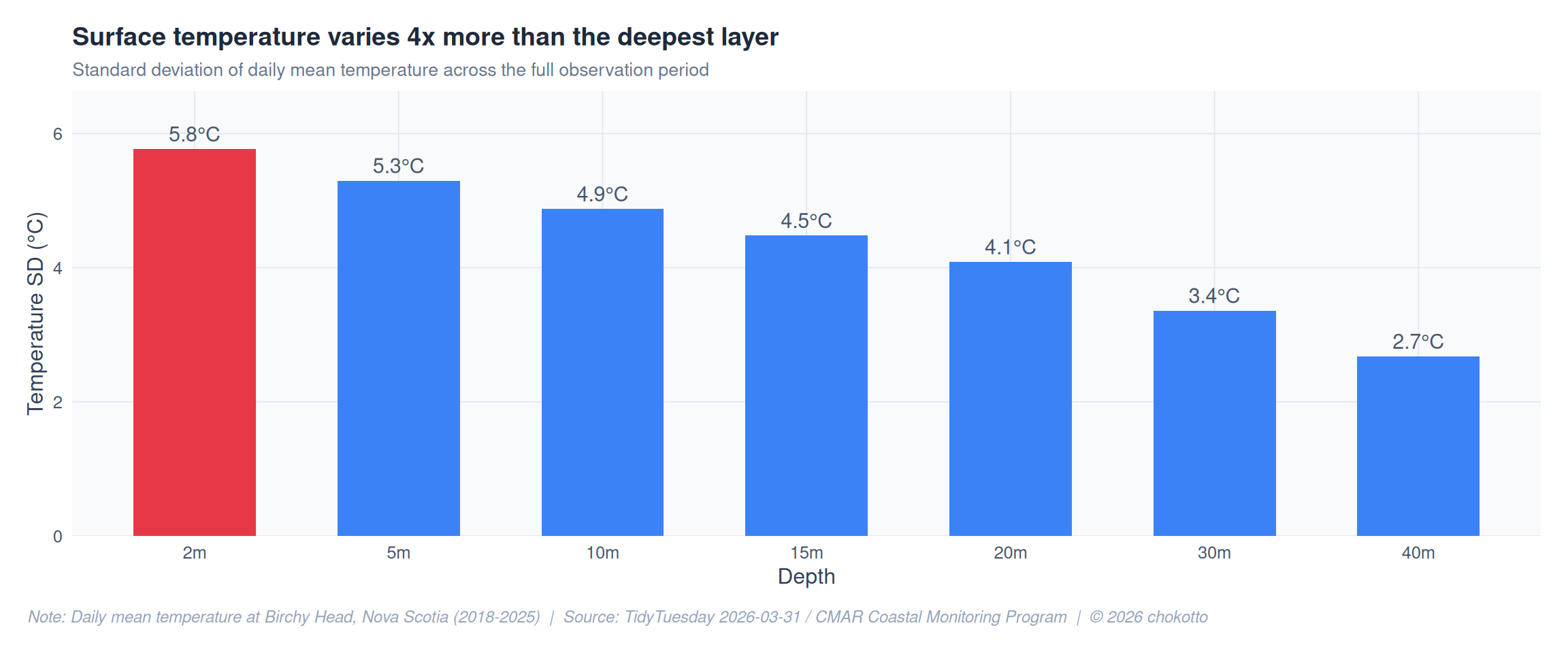
The ocean has a thermal memory. Surface waters (2m) swing 20+ degrees C across seasons, but the 40m layer remains nearly constant, buffered by thermal stratification.
Summer warmth barely reaches 20m. The seasonal pulse attenuates sharply with depth. Below 20m, the annual temperature range compresses to just a few degrees.
Variability decreases monotonically with depth. The standard deviation of daily temperatures at 2m is roughly 4x that at 40m, confirming that deeper waters act as thermal stabilizers.
Year-to-year variation is most visible at the surface. Inter-annual differences in annual mean temperature are larger at shallower depths, suggesting surface layers are more responsive to atmospheric forcing.
This post is part of the TidyTuesday weekly data visualization project.