TidyTuesday: Bird Sightings at Sea - New Zealand Logbooks

Seabird counts from 10-minute ship surveys near New Zealand (1969-1990): species, season, wind, and geography

Overview

This week we explore seabird observations recorded under the Australasian Seabird Mapping Scheme: counts from ships during 10-minute periods near New Zealand waters. The data links bird records to ship position, weather, and season.

• Data Source: TidyTuesday 2026-04-14 / Te Papa Tongarewa
• Angle: Which species dominate counts, how observations vary by season and wind, and where surveys cluster in space

Dataset

library(tidyverse)
library(scales)
library(glue)
library(patchwork)
library(ggtext)
library(ggrepel)
library(showtext)
library(colorspace)
library(janitor)
library(forcats)

birds_path <- file.path(getwd(), "data", "birds.csv")
ships_path <- file.path(getwd(), "data", "ships.csv")
base_url <- "https://raw.githubusercontent.com/rfordatascience/tidytuesday/main/data/2026/2026-04-14"

if (!file.exists(birds_path)) {
  birds_path <- paste0(base_url, "/birds.csv")
}
if (!file.exists(ships_path)) {
  ships_path <- paste0(base_url, "/ships.csv")
}

birds <- readr::read_csv(birds_path, show_col_types = FALSE, na = c("", "NA"))

Warning: One or more parsing issues, call `problems()` on your data frame for details,
e.g.:
  dat <- vroom(...)
  problems(dat)

ships <- readr::read_csv(ships_path, show_col_types = FALSE)

birds_ship <- birds |>
  inner_join(ships, by = "record_id") |>
  mutate(
    species_label = coalesce(species_scientific_name, species_common_name, "Unknown"),
    count = replace_na(count, 0L)
  ) |>
  filter(!is.na(species_label), species_label != "Unknown")

beaufort_path <- file.path(getwd(), "data", "beaufort_scale.csv")
if (!file.exists(beaufort_path)) {
  beaufort_path <- paste0(base_url, "/beaufort_scale.csv")
}
beaufort <- readr::read_csv(beaufort_path, show_col_types = FALSE)

NOTE_TEXT   <- "Seabird logbook entries; counts may be censored at 99999 for very large flocks"
SOURCE_TEXT <- "TidyTuesday 2026-04-14 / Te Papa Tongarewa"
CAPTION     <- glue("Note: {NOTE_TEXT}  |  Source: {SOURCE_TEXT}  |  \u00A9 2026 chokotto")

STYLE_MODE <- "figmamake"

theme_fm <- theme_minimal(base_size = 12) +
  theme(
    plot.background = element_rect(fill = "white", color = NA),
    panel.background = element_rect(fill = "#f8fafc", color = NA),
    panel.grid.major = element_line(color = "#e2e8f0", linewidth = 0.3),
    panel.grid.minor = element_blank(),
    text = element_text(color = "#334155"),
    axis.text = element_text(color = "#475569"),
    plot.title = element_text(color = "#1e293b", face = "bold", size = 14),
    plot.subtitle = element_text(color = "#64748b", size = 10),
    plot.caption = element_text(
      face = "italic", color = "#94a3b8", size = 9,
      hjust = 0, margin = margin(t = 12)
    ),
    plot.caption.position = "plot",
    strip.text = element_text(color = "#1e293b", face = "bold"),
    legend.background = element_rect(fill = "white", color = NA),
    legend.text = element_text(color = "#475569"),
    plot.margin = margin(15, 15, 15, 15)
  )

theme_active <- theme_fm

COL_PRIMARY   <- "#0ea5e9"
COL_SECONDARY <- "#f59e0b"
COL_ALERT     <- "#ef4444"
COL_POSITIVE  <- "#10b981"
COL_BASE      <- "#94a3b8"

Analysis

Albatrosses and petrels lead the species list

species_tot <- birds_ship |>
  group_by(species_label) |>
  summarise(total_count = sum(count, na.rm = TRUE), n_obs = n(), .groups = "drop") |>
  filter(total_count > 0) |>
  slice_max(total_count, n = 15) |>
  mutate(species_label = fct_reorder(species_label, total_count))

ggplot(species_tot, aes(x = total_count, y = species_label)) +
  geom_col(fill = COL_PRIMARY, width = 0.7, alpha = 0.85) +
  geom_text(
    aes(label = comma(total_count)),
    hjust = -0.1, size = 3, color = "#475569"
  ) +
  scale_x_continuous(labels = comma_format(), expand = expansion(mult = c(0, 0.12))) +
  labs(
    title = "Top seabird taxa by summed count in the survey window",
    subtitle = "15 species with highest total birds recorded (all observations combined)",
    x = "Total birds counted",
    y = NULL,
    caption = CAPTION
  ) +
  theme_active +
  theme(panel.grid.major.y = element_blank())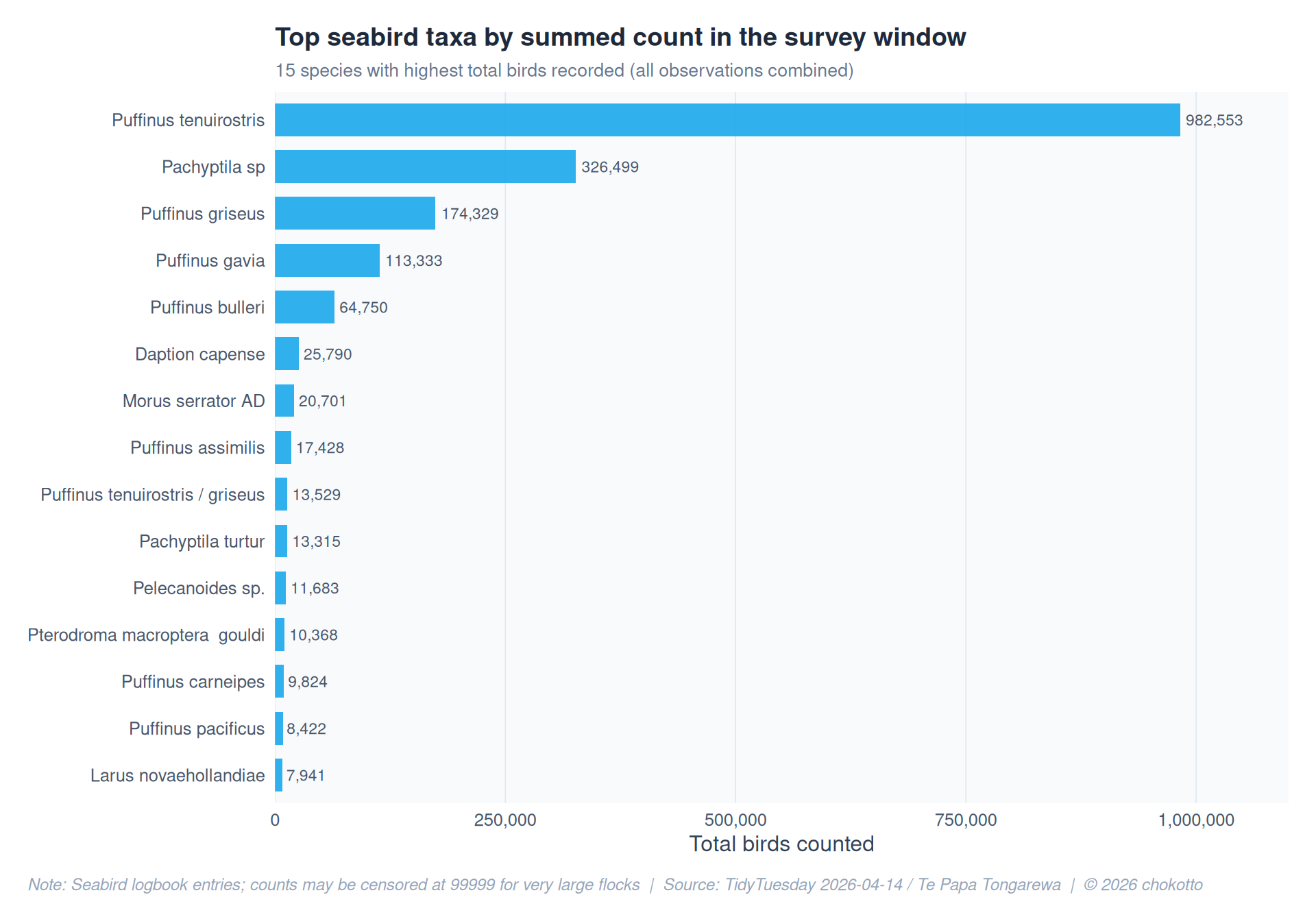

Summer surveys capture the most activity

season_n <- birds_ship |>
  filter(!is.na(season)) |>
  count(season, name = "n_records")

ggplot(season_n, aes(x = season, y = n_records, fill = season)) +
  geom_col(width = 0.65, show.legend = FALSE) +
  scale_fill_manual(
    values = c(
      "summer" = COL_PRIMARY,
      "autumn" = COL_SECONDARY,
      "winter" = lighten(COL_ALERT, 0.2),
      "spring" = COL_POSITIVE
    )
  ) +
  scale_y_continuous(labels = comma_format()) +
  labs(
    title = "Observation records peak in southern summer",
    subtitle = "Number of bird records linked to ship logs by hemisphere season",
    x = NULL,
    y = "Number of records",
    caption = CAPTION
  ) +
  theme_active +
  theme(panel.grid.major.x = element_blank())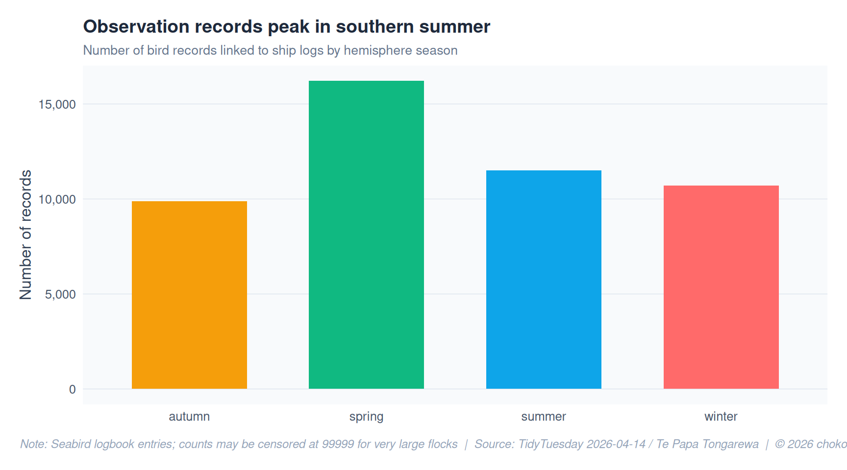

Higher wind classes still show heavy bird activity

wind_df <- birds_ship |>
  filter(!is.na(wind_speed_class)) |>
  group_by(wind_speed_class) |>
  summarise(
    mean_count = mean(count, na.rm = TRUE),
    n = n(),
    .groups = "drop"
  ) |>
  left_join(
    beaufort |> select(wind_speed_class, wind_description),
    by = "wind_speed_class"
  )

ggplot(wind_df, aes(x = factor(wind_speed_class), y = mean_count)) +
  geom_col(fill = lighten(COL_SECONDARY, 0.25), width = 0.65) +
  geom_text(
    aes(label = comma(round(mean_count, 1))),
    vjust = -0.4, size = 3, color = "#475569"
  ) +
  labs(
    title = "Mean flock size by Beaufort wind class",
    subtitle = "Higher classes are rougher seas; counts remain substantial across conditions",
    x = "Beaufort wind class",
    y = "Mean birds per observation",
    caption = CAPTION
  ) +
  theme_active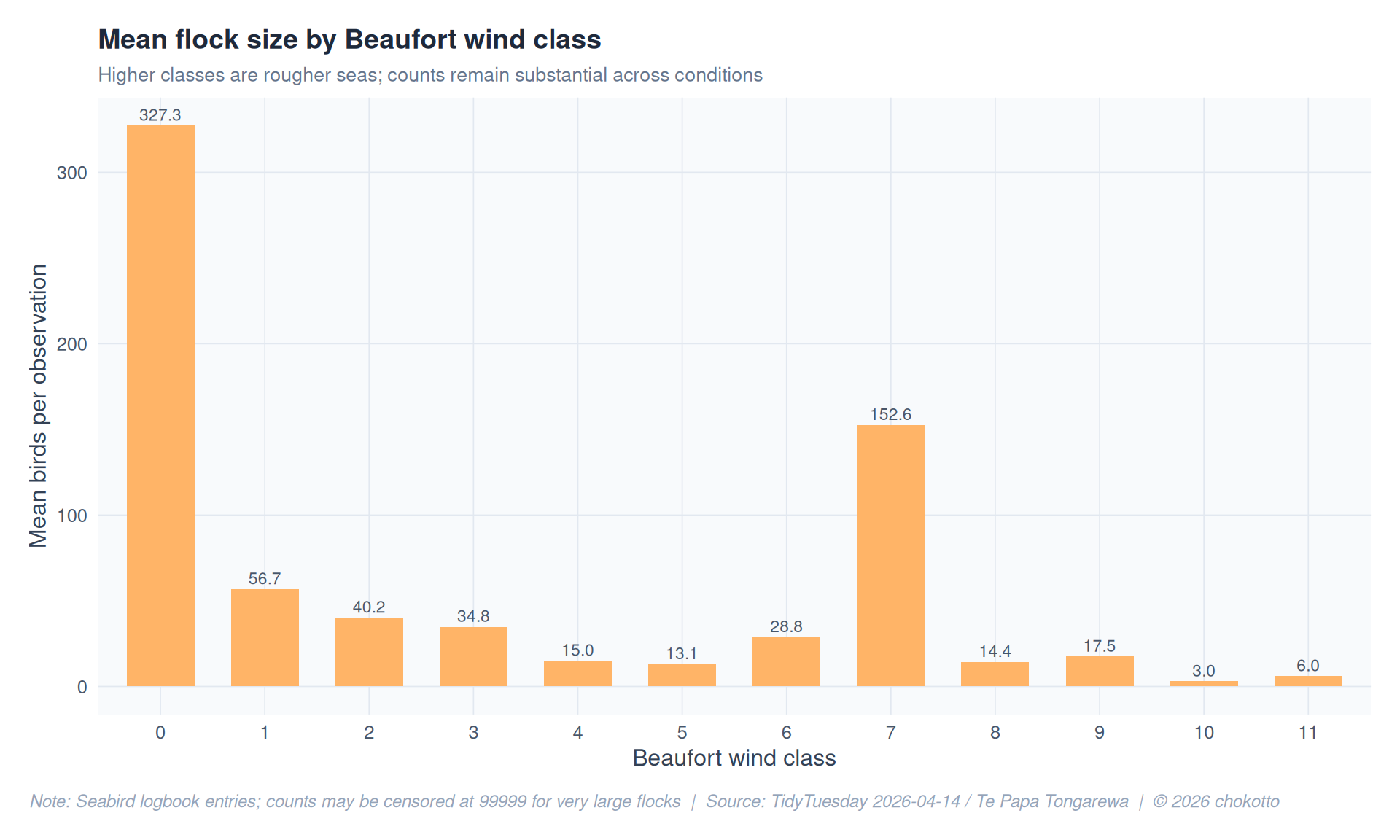

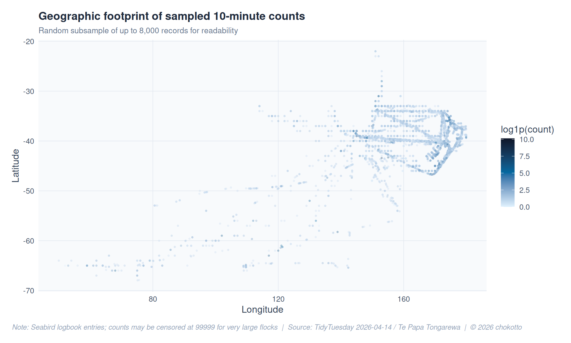
Surveys trace a belt of observations around New Zealand waters

set.seed(42)
map_df <- birds_ship |>
  filter(!is.na(latitude), !is.na(longitude))

# slice_sample(n = min(8000, n())) fails: inside slice_sample(), n() is not nrow(.)
if (nrow(map_df) > 0L) {
  n_map <- min(8000L, nrow(map_df))
  map_df <- slice_sample(map_df, n = n_map)
}

if (nrow(map_df) == 0L) {
  ggplot() +
    annotate(
      "text", x = 0.5, y = 0.5, size = 4, color = "#64748b",
      label = "No latitude/longitude available for mapping."
    ) +
    theme_void()
} else {
  ggplot(map_df, aes(x = longitude, y = latitude)) +
    geom_point(aes(color = log1p(count)), alpha = 0.25, size = 0.6) +
    scale_color_gradientn(
      colors = c("#e0f2fe", "#0369a1", "#0f172a"),
      name = "log1p(count)"
    ) +
    labs(
      title = "Geographic footprint of sampled 10-minute counts",
      subtitle = "Random subsample of up to 8,000 records for readability",
      x = "Longitude",
      y = "Latitude",
      caption = CAPTION
    ) +
    theme_active +
    theme(legend.position = "right")
}

Key Findings

• Large albatross and petrel aggregates drive the highest summed counts, reflecting both abundance and schooling behavior in the Southern Ocean survey corridor.
• Southern summer contains the bulk of linked records, consistent with more research and fishing vessel activity in warmer months.
• Wind conditions span calm to rough seas; mean per-observation counts stay meaningful even at higher Beaufort classes.
• Spatially, observations concentrate in a band consistent with New Zealand’s offshore and subantarctic routes.

---

This post is part of the TidyTuesday weekly data visualization project.

CautionDisclaimer

This analysis is for educational and practice purposes only. Data visualizations and interpretations are based on the provided dataset and may not represent complete or current information.